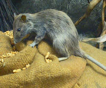
 Maybe the rats are not the source of the "Black Death" in the 14th century. (c)wikimedia.commons Maybe the rats are not the source of the "Black Death" in the 14th century. (c)wikimedia.commons I learned in school that in the 14. century the “Black Death” plague was caused by the bacterium Yersinia pestis which was transmitted by rat fleas. However, this may not be true. So yes, plague is caused by Yersinia pestis, but there are different infection ways: (I) from rat fleas to human, (II) from human ectoparasites (fleas and lice) to human and (III) from human to human by inhalation from infected droplets. But how you can find out many centuries later which infection way was the basis for the “Black Death”? The answer is: with mathematical models! Katharine R. Dean, et al. (PNAS 2018) created mathematical models for all three infection ways. So they were able to simulate how infection rates would develop over time for each type of infection. Then they fitted the simulation results to real outbreak data and showed that in many cases the “human ectoparasites to human” model fits best. Of course, it can still be that it was a mixture of different infection ways and that the main infection way differed from region to region. Nevertheless, it shows that the story which we learn in school, that the plague is caused by infected rats and rat fleas, is maybe too easy.
0 Kommentare
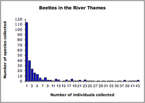 Example for a hollow curve distribution. (c)wikipedia: derived from data presented in Magurran (2004) and collected by Williams (1964) Example for a hollow curve distribution. (c)wikipedia: derived from data presented in Magurran (2004) and collected by Williams (1964) A large variety of life exists on earth. Biologists sort this biodiversity in a hierarchical system of taxonomic ranks: species, genus, family and so on. Interestingly, “at any taxonomical level, a very small number of units have a very large number of subunits, e.g., individuals per species, or genera per family, followed by a very rapid dropoff, resulting in what is commonly called a hollow curve distribution.” (Beres, et al. 2005). How does this unequal distribution evolve? Normally, when we talk about evolution and origin of biodiversity, we think about “survival of the fittest”, and mutations which help to adapt to different niches, … . However, in order to reproduce the hollow curve distribution (with mathematical models) you don’t need to assume differences in fitness and survival rate. The so called (Hubbell’s) “unified neutral theory of biodiversity” assumes that death and reproduction rates is independent from individual’s species and its neighbourhood. You fix the amount of individuals for an area (“zero-sum” assumption). The individuals can belong to different species. Every time step you pick randomly on of the individuals which has to die. At the same time you choose randomly on of the individuals who reproduces itself to fill the new gap. Moreover, there is a chance that the new individual evolves to a new species which balances random extinction and allows the number of species to stabilise. Of course there are different versions of that theory, more or less complicated, which were fitted to different datasets describing distributions e.g. of tree or coral species. But I want to point out (and what fascinates me about this topic) is that these simple assumptions/rules are all you do not need in order to reproduce the measured hollow curve distributions: No survival of the fittest but simple random events of death and reproduction and some mutations. Egbert G Leigh Jr. et al. (2010), Scholarpedia, 5(11):8822.
"The unified neutral theory of biodiversity and biogeography at age ten." James Rosindell, Stephen P. Hubbell, and Rampal S. Etienne. Trends in ecology & evolution 26.7 (2011): 340-348. "Rotifers and Hubbell's unified neutral theory of biodiversity and biogeography." Karl A. Beres, Robert L. Wallace, and Hendrik H. Segers. Natural Resource Modeling 18.3 (2005): 363-376.  A beech leaf is (similar to all common leaves) flat with a upper and a lower side. This asymmetric shape is created by differences in cell wall stiffness. (photo (c): wikipedia) A beech leaf is (similar to all common leaves) flat with a upper and a lower side. This asymmetric shape is created by differences in cell wall stiffness. (photo (c): wikipedia) Welcome back from the fall vacation break. Did you ever wonder how a leaf becomes its leaf form? Jiyan Qi et al (2017) had this question and wrote a paper about it. We know that a leaf is constructed by different tissues/parts: because of differences in gene expression the upper side (adaxial domain) looks different from the lower side (abaxial domain). But which mechanism creates the flat leaf form with upper and lower side? The bud… ergo the start of a developing leaf… is round! Jiyan Qi et al (2017) showed that “relatively simple changes in mechanical properties can account for dynamic shape changes during asymmetric leaf development”. To make a long story short: In the developing (round) leaf the lower side has a higher auxin concentration as the upper side. Auxin is a plant hormone and can lead for example to cell wall loosening by de-methyl-esterification of pectins, a major component of the primary cell wall. The lower sider gets more elastic as the upper side. This difference in elasticity leads to the leaf asymmetry. With proceeding development, the rigid zone of the upper side moves to the middle. “From a physical perspective, the stiff cells receive stronger constraints from their neighbouring […] cells, such that they prefer to grow and divide by pressing on the soft inner cells“. The leaf stretches and gets flat. Just as side note: What I like about the paper is that they use computational models to test their hypothesis if differences in cell wall stiffness and epidermal restriction can lead to the leaf asymmetry. They model what would happen if the cell wall elasticity of the upper and lower region is changed/mixed up. Then they test the model predictions by manipulating the cell wall plasticity experimentally. 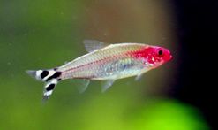 Red nose tetra fish group organization depends on the swimming speed. (c)wikimedia Red nose tetra fish group organization depends on the swimming speed. (c)wikimedia In 1973, D. Weihs modelled fish schools and predicetd that the diamond shape (shifted rows, so that the single fish is always in the middle between the two nearest neighbours in front of it) is the preferred organization structure. He could show by 2D modelling, that the diamond shape could improve swimming efficiency because of the hydrodynamic interactions with the vortices created by the fishes in front. Intesaaf Ashraf et al. (2017) challenge this widespread idea of prefered diamond shape organization. They studied fish schools of the red nose tetra fish (Hemigrammus bleheri) and showed that the organization structure depends on the swimming speed. Slow swiming fishgroups showed indeed a preference for diamond or T-shape organization. However, when forced to swim faster, so in a situation in which energy efficiency would be most beneficial (for example when escaping a predator), they prefer a “in line” (phalanx-shaped) organization. This phalanx pattern reduces the distance to to the nearest neighbour. Both configurations, diamond-shaped and phalanx-shaped, save energy (reducing tail-flapping frequency) compared to a single fish swimming alone. So why changing to a line when fast swimming is required? Ashraf et al. think this conformation change is connected to the change of swim-movement-synchronization. While slow swimming fishes show no correlation in their tail movement, fast swiming fishes were synchronized (in phase or out-of phase) with their nearest neighbour. Ashraf et al. predict that this synchronized swimming kinetics together with the “side by side” organization is a good strategy to optimize thrust (and therefore speed). Unfortunately, they didn’t modeled this configuration to proof this idea. However, this study shows that maybe Weihs model of energy-saving diamond-shaped fish schools maybe needs some improvement. “Simple phalanx pattern leads to energy saving in cohesive fish schooling“
I. Ashraf et al. (2017) PNAS, doi:10.1073/pnas.1706503114 Copper… on the one hand copper is an important trace element for life (for example as part of the red blood cells), on the other hand it is toxic. Water-soluble copper in inshore waters and soil is a danger for many microorganisms and plants. Therefore, it is important to understand the dispersion of water-soluble copper. When you add water-soluble copper (Cu) into soil, it instantly partitions between solid and solution phases. However, this state is not stable: with increasing “age”, its lability (bioavailability, toxicity, isotopic exchange-ability and extractability) decreases because of diffusion and reactions with the surrounding material. Theoretical models help to predict this time dependent change in lability, which depends on a lot of soil parameters like temperature, soil organic matter content and soil pH. Zeng, et al. (2017) published an improved model for copper lability which describes short and long term effect of water-soluble copper added to soil in one single model. In their model, copper lability depends on three processes:
The model showed good predicting ability when compared to experimental data of different soil samples with different chemical properties (like pH value, clay and organic carbon content and copper concentration), although other copper ageing processes like moisture, plant absorption, and microbial activities are not considered. "A new model integrating short- and long-term aging of copper added to soils"
Zeng S, Li J, Wei D, Ma Y (2017) PLOS ONE 12(8): e0182944. As you may now, biological cells consist of a variety of “walls” (membranes) which form the outer borders and separate internal compartments (“rooms” for energy production, reproduction, transport,…). In these walls there are “doors”/tunnels (channels, pumps,…) which allow molecules to pass through. However, in order to guarantee the function of the cell, it is important to control the flux of molecules and therefore many tunnels are selective for a certain type of molecules. Meaning: just certain molecules can cross through the tunnel and other molecules can not. How is this achieved? Even if there is just the right molecule around, the probability of that molecule to find this tunnel by random motion is quite low. However, in the biological cell there are thousands of different types of molecules. So the probability of the tunnel to “find” the right molecule and let it pass to the other side of the “wall” should be even lower. No! Anton Zilman et al. (2010) found out (with the help of a theoretical model and proved by experiments) that the transport probability of the tunnel-specific molecules can actually increase in the presence of non-specific molecules. To understand this, it is important to remember that the molecules move random. Inside the tunnel they may attach to it which allows them to “stay in place” for a short time, but every molecule will move at sometime in a random direction. Therefore, entering the tunnel doesn’t mean that the molecule will “walk” through the tunnel and left it on the other side of the “wall”. Another important point is that the space in the tunnel is limited. Meaning, every “spot” in the tunnel just has space for a fixed number of molecules attaching to it. The point with the selectivity is then controlled by the difference in how long a molecule can attach to the tunnel. So tunnel-specific molecules can attach longer and so can “stay” longer in the tunnel before they move randomly compared to non-specific molecules. Anton Zilman et al. (2010) created a model for the tunnel and simulated the movements of two competing molecule types (one better attaching to the tunnel than the other). The tunnel itself was divided in “spots”… so a longer tunnel has more “spots” a molecule has to cross on its way than a short tunnel. A molecule just moves to a neighboring spot when there is a free place (as said before, the “diameter” of the tunnel restricts how many molecules can be on the same place at the same time). The better attaching moecules can stay longer on a spot than then non-specific molecules. So what is happening: If the non-specific molecules have a really short attaching time, because the binding between molecule and tunnel is weak, then it does not affect the transport of the strong binding (long attaching) molecules because it has already problems to reach the entrance. In the other hand, when both molecules have strong binding, the “wrong” (non-specific) molecule can block the entrance and the transport of the specific molecule is decreased. However, if the non-specific molecule has an intermediate attaching time, it can enhance the transport of the specific molecule. The intermediate binding strength allows the non-specific molecules to enter the entrance. This hinders the return of the specific molecules which are already in the channel and so the latter “has to” go in the right direction and cross the tunnel instead of going backwards. A little bit counter intuitive, isn’t it? Just imagine there is a real tunnel and there are two types of people: one type is really fascinated by tunnel walls. They love to look at it in detail and so spend a lot of time in the tunnel while walking slowly in a random direction (because they are so distracted that they don’t know in which direction they are walking). Now you add a second type of people: people which are not afraid of tunnels and are curious but they are not so fascinated and so are moving much faster and defer to the type one people regarding a spot in the tunnel. The fascinated people will go deep in the tunnel while the hectic people stay near the entrance. The hectic people in the entrance do not hinder the fascinated people to enter the tunnel. However, as the hectic people are crowding the entrance, it is much easier for the fascinated people to walk through the tunnel instead of returning to the entrance. Therefore, more fascinated people are walking through the tunnel as it would be without the hectic people. Enhancement of Transport Selectivity through Nano-Channels by Non-Specific Competition
Anton Zilman et al. PLoS Comput Biol 6.6 (2010): e1000804. 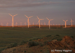 The best “papers of the day” are papers which deal with problems I never thought about although they are quite obvious. This is the case for the paper of Amr M. Abd-Elhady et al. (2014) which deals with the problem of backflow current-overvoltages in wind turbines. I never thought about it, but wind turbines have a high risk of being hit by a lightning due to their size and location. Of course, wind turbines have a grounding system. However, that grounding system depends on the soil resistivity (= how much the soil resists the flow of electricity) which depends on moisture and salt content and temperature. High soil resistivity makes it “difficult to attain low grounding impedance for the utilized electrodes. These increase the ground potential rise (GPR) and make surge arresters operate in reverse direction.” The resulting backflow surge current can damage the equipment (cable, transformers, surge arresters . . .) and therefore needs to be prevented. Using a modelling approach, Amr M. Abd-Elhady et al. analysed which parameters influence the damage caused by lightning and tested an alternative grounding system. For example: The lightning damage is worse when the lightning hits the wind turbine at the negative peak of voltage waveform. Moreover, they compared the damage in “in service” and “out of service” wind turbines and the influence of the number of connected wind turbines in a wind farm. Interestingly, the damage decreases with increasing the number of wind turbines for the non-thunderstruck turbines case and increases with increasing the number of wind turbines for the thunderstruck turbines. So in larger wind farms, the wind turbine which is hit by lightning receives more damage but the surrounded wind turbines are less damaged compared to a small wind farm. High-frequency modeling of Zafarana wind farm and reduction of backflow current-overvoltages
Amr M. Abd-Elhady, Nehmdoh A. Sabiha and Mohamed A. Izzularab International Transactions on Electrical Energy Systems 24.4 (2014): 457-476. 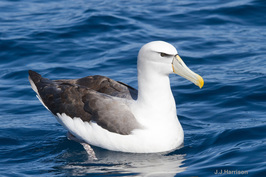 This bird has nothing to do with the activity-based ALBATROSS model This bird has nothing to do with the activity-based ALBATROSS model Air quality is a main problem of the civilization. Therefore, models predicting air pollution become more and more important. And this is quite easy. Let Aurora work together with albatross, and you will get good predictions. Of course I am referring to the paper of Carolien Beckx et al. (2009) and ALBATROSS and AURORA are models: A Learning-Based Transportation Oriented Simulation System and Air quality modelling in Urban Regions using an Optimal Resolution Approach. ALBATROSS is an activity-based model which predicts people's travel behaviour and the resulting vehicle emissions. It is based on approximately 10,000 person-day activity-diaries of Dutch. The predictions of vehicle emissions can be used as input for the air quality model AURORA. As “prognostic 3-dimensional Eulerian model of the atmosphere”, AURORA predicts how air pollutants (gas and particla) are transported in the air, including physical changes and chemical reactions which generate new pollutants. Using meterological parameters like wind, temperature, humidity, precipitation, radiation,…, AURORA calculates 3-dimensional concentration fields for different pollutants. Beckx et al. (2009) tested this model combination by comparing the model predictions for three different pollutants with real air quality data measured in different stations all over the Netherlands. Inside the country, the agreement between modelled and observed concentrations varied between the different pollutants but was sufficient for all of them. The only problems are the borders of the Netherlands, maybe because of wrong calculation of the contribution of foreign traffic. Maybe they underestimated how many people like to visit the Netherlands? The contribution of activity-based transport models to air quality modelling: a validation of the ALBATROSS–AURORA model chain
Carolien Beckx, et al. Science of the Total Environment 407.12 (2009): 3814-3822 |
IdeaI love to increase my general science knowledge by reading papers from different fields of science. Here I share some of them. Archiv
März 2018
Kategorien
Alle
|
 RSS-Feed
